The Beatles became a hit through its sometimes simple but always powerful music but it has never been famous for its poetry. The group’s lyrics, however, did change during the band’s short existence and we can use text analysis to track these changes. This post is about measuring the change in the complexity of the group’s lyrics, from the Please, Please Me to the Abbey Road albums, showing how we can use basic data secience tools to find really fancy patterns in unstructured text data.
This piece is a shortened version of a final project for a Data Science on Unstructured Text Data course held by Facebook’s Eduardo Ariño de la Rubia. The course introduced the tidytext package and the basics of text analysis in R. At the end of the course students had to present their skills through a freely chosen analysis project. Although tidytext does not directly cover text complexity, to me it was somehow an obvious choice.
This is a technical post, but most of the hard stuff is concentrated in the code blocks. If you are only interested in the power of data science, feel free to disregard these blocks and concentrate on the text and the plots only. You will still be able to get the message.
When you learn English as a foreign language you inevitably bump into The Beatles early on. The songs are well known, and even a beginner student can easily understand the lyrics. This is not only because the members were singing in nice English, but because their early text is damned simple. ‘She loves you, yeah, yeah, yeah.’ Not that of a challenging text, right?
But when you listen to The Beatles a little more, you realize that as time went by their songs got more and more sophisticated. ‘Strawberry Fields Forever’ does have more depth than ‘A Hard Day’s Night’. Since we are into data science, it is obvious to ask: can we measure this change in sophistication? Can we trace the development also in their lyrics? As the members went from their early twenties towards their thirties, did they move from their simple but powerful origins towards something more mature?
In the next few lines I am analyzing The Beatles’ thirteen albums of ‘core catalogues’ from ‘Please Please Me’ to ‘Let It Be’, published between 1964 and 1970. It is amazing but the most influential pop group of all times existed for less than a decade, and this short period was enough to issue thirteen albums and to turn the world upside down. The group had quite a few extra collections, live recordings and greatest hit compilations (the last one, according to wikipedia, in 2013), but these thirteen albums make up the the actual works of the group.
For the project I used the newly developed geniusR package by Josiah Parry, which downloads lyrics and
metadata from the genius.com homepage. This package was of enormous help
for the analysis.
A Glance At The Beatles
As a starter I imported the necessary packages. I like starting all analysis with the packages, having them in one single chunk for a better overview. Also, when I later need to add further packages I just scroll back to the first chunk to enter the extra library command.
library(geniusR)
library(tidyverse)
library(tidytext)
library(tidyr)
library(tibble)
library(dplyr)
library(purrr)
library(stringr)
library(syllable)
library(ggplot2)
library(scales)
library(gridExtra)
library(lsa)
library(rlist)
library(data.table)
Downloading the text is simple with geniusR: you define the artist, the number of albums to download, and the album titles. Album titles should be entered as the last part of the urls on the genius.com webpage without hyphens. Apostrophes are omitted. You can also download albums of multiple artists entering the author, # of albums multiple times as a vector. See the documentation and Josiah’s github for details.
It takes a while until your text downloads, but you end up with a nice (tidy!) tibble which serves as the basis for further analysis.
albums <-  tibble(
  artist =
    rep("The Beatles", 13),
  album = c(
    "Please Please Me", "With The Beatles", "A Hard Day s Night",
    "Beatles For Sale", "Help", "Rubber Soul",
    "Revolver", "Sgt Pepper s Lonely Hearts Club Band", "Magical Mystery Tour",
    "The Beatles The White Album", "Yellow Submarine", "Abbey Road",
    "Let It Be"
  )
)

album_lyrics <- albums %>%
  mutate(tracks = map2(artist, album, genius_album))

beatles_lyrics <- album_lyrics %>%
  unnest(tracks)

beatles_albums <- beatles_lyrics %>%
  distinct(album)
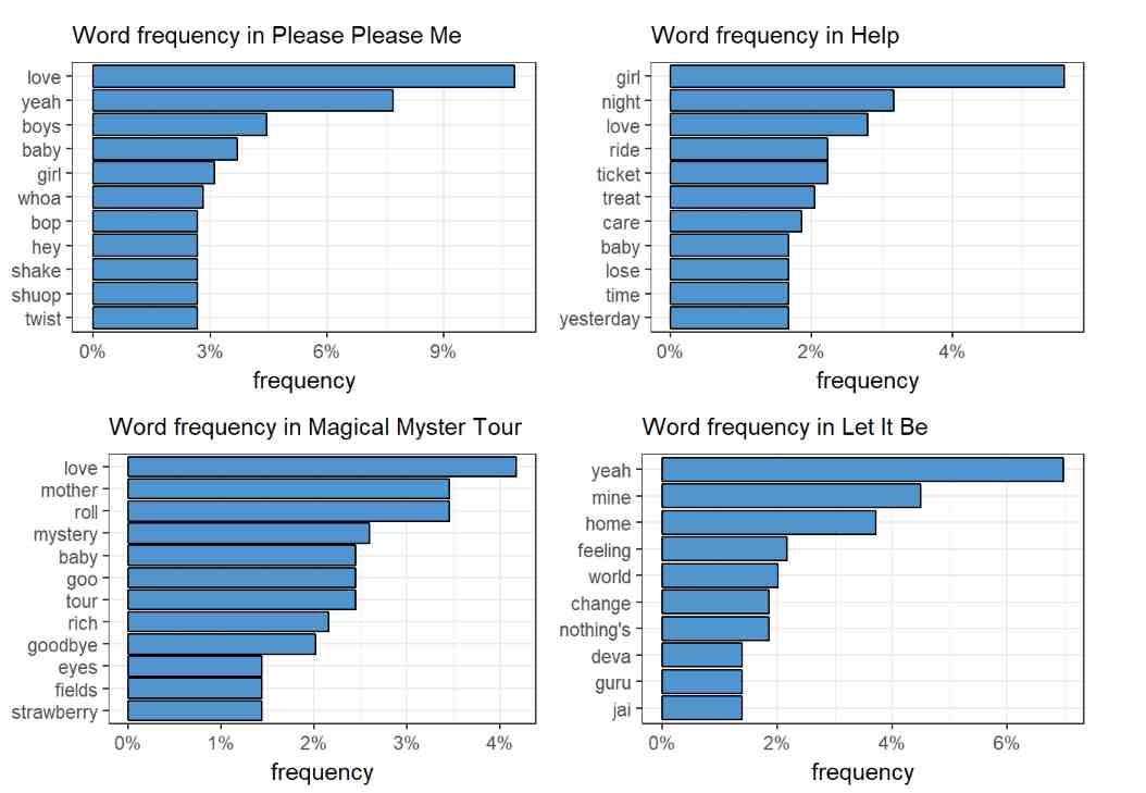
As the most obvious starting point of any text analysis, I checked the per album frequencies of non-stop words across these albums. (For the wider audience: stop words are the most common, ‘functional’ words in a language.) In order to draw an arch of change, I plotted simple word frequency charts for Please Please Me (1963), Help (1965), Magical Mystery Tour (1967) and Let It Be (1970). Can we see any difference in the words used?
tidy_beatles <- beatles_lyrics %>%
  unnest_tokens(word, text) %>%
  filter(nchar(word)>2)%>%
  anti_join(stop_words) %>%
  group_by(album) %>%
  count(word, sort = TRUE) %>%
  ungroup()

total_words <- tidy_beatles %>%
  group_by(album) %>%
  summarize(total = sum(n))

tidy_beatles <- left_join(tidy_beatles, total_words)

tidy_beatles <- tidy_beatles %>%
  mutate(freq = n / total)

ppm <- tidy_beatles %>%
  filter(str_detect(album, "Please"))%>%
  arrange(desc(freq)) %>%
  top_n(10)%>%
  mutate(word = factor(word, levels = rev(unique(word)))) %>%
  ggplot(aes(word, freq, fill=I("steelblue3"), col=I("black"))) +
  geom_col(show.legend = FALSE) +
  labs(x = NULL, y = "frequency") +
  coord_flip() +
  theme_bw() +
  labs(title = "Word frequency in Please Please Me") +
  theme(plot.title = element_text(size = rel(1))) +
  scale_y_continuous(labels = percent)

help <- tidy_beatles %>%
  filter(str_detect(album, "Help"))%>%
  arrange(desc(freq)) %>%
  top_n(10)%>%
  mutate(word = factor(word, levels = rev(unique(word)))) %>%
  ggplot(aes(word, freq, fill=I("steelblue3"), col=I("black"))) +
  geom_col(show.legend = FALSE) +
  labs(x = NULL, y = "frequency") +
  coord_flip() +
  theme_bw() +
  labs(title = "Word frequency in Help") +
  theme(plot.title = element_text(size = rel(1))) +
  scale_y_continuous(labels = percent)

mys <- tidy_beatles %>%
  filter(str_detect(album, "Mystery"))%>%
  arrange(desc(freq)) %>%
  top_n(10)%>%
  mutate(word = factor(word, levels = rev(unique(word)))) %>%
  ggplot(aes(word, freq, fill=I("steelblue3"), col=I("black"))) +
  geom_col(show.legend = FALSE) +
  labs(x = NULL, y = "frequency") +
  coord_flip() +
  theme_bw() +
  labs(title = "Word frequency in Magical Myster Tour") +
  theme(plot.title = element_text(size = rel(1))) +
  scale_y_continuous(labels = percent)

lib <- tidy_beatles %>%
  filter(str_detect(album, "Let"))%>%
  arrange(desc(freq)) %>%
  top_n(10)%>%
  mutate(word = factor(word, levels = rev(unique(word)))) %>%
  ggplot(aes(word, freq, fill=I("steelblue3"), col=I("black"))) +
  geom_col(show.legend = FALSE) +
  labs(x = NULL, y = "frequency") +
  coord_flip() +
  theme_bw() +
  labs(title = "Word frequency in Let It Be") +
  theme(plot.title = element_text(size = rel(1))) +
  scale_y_continuous(labels = percent)

grid.arrange(ppm, help, mys, lib, nrow = 2)

Love makes it into the first 10 in three of the albums, leading the pack in Please Please Me and, to my little surprise, Magical Mystery Tour. Interestingly, it is missing from the top 10 in Let It Be, the last album. It looks, love was not of primary interest by 1970, the year when the members decided to go their own separate ways. Of course, per album word frequency depends largely on the songs’ topic selection: ‘mother’ goes to number 2 in Magical Mystery Tour due to the many repetitions of the line ‘Your mother should know’ in the song of the same title.
This simple exercise shows that working with lyrics can be very tricky.
Lines are repeated very often, and melody dominates sentence building.
As a matter of fact, sentences can only be poorly defined by regular
text analysis algorithms in songs, which, as we will see later, makes
measuring text complexity somewhat difficult.
Measuring Similarity Across Core Albums
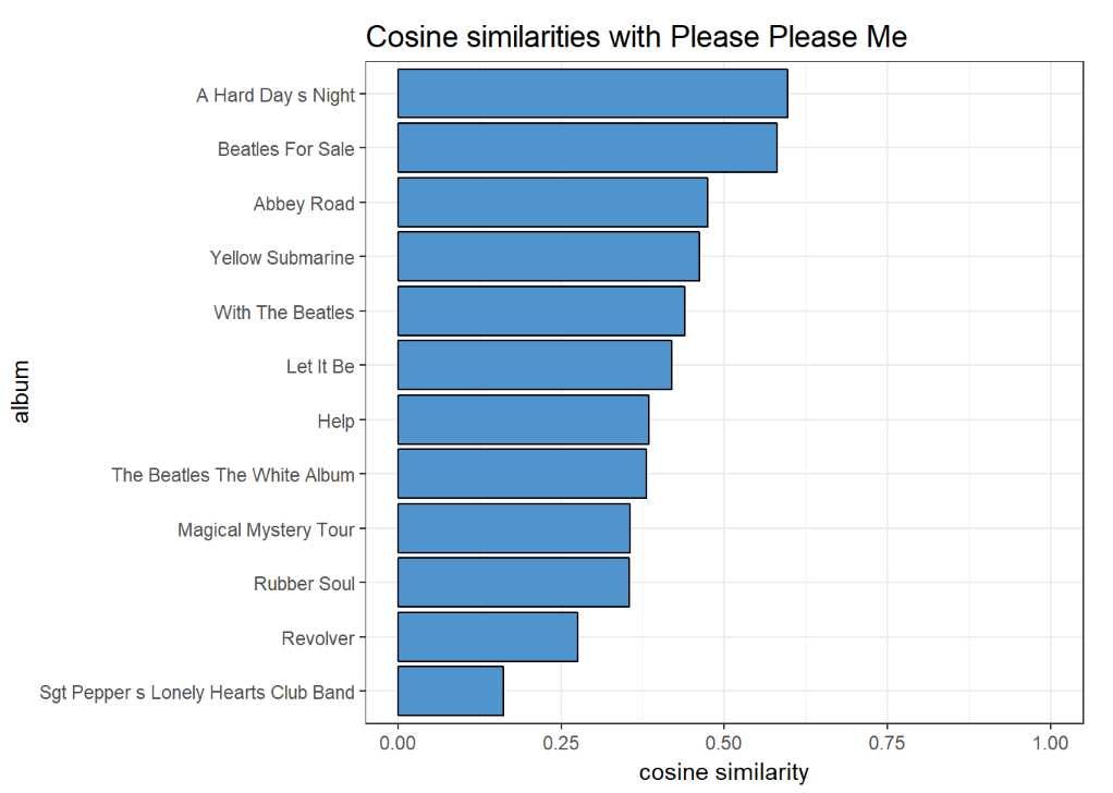
In order to asses how much the group changed over the course of these seven years I measured the similarity of each album to Please Please Me, the very first LP. More and more sophisticated lyrics would result in larger and larger differences in text, measured by cosine similarity.
I calculated cosine similarity based on word frequency vectors, where each album is vector of frequencies of words in a union of sets of words from each album. The word list is a product of a full join of all words from the all the albums, and the cosine for each album is a similarity measure between that particular album and the benchmark Please Please Me. This word list excludes stop words, of course.
cos <- tidy_beatles %>%
  select(album, word, freq)

cos_w <- spread(cos, key = album, value = freq) # This is a matrix where entries are frequencies of words in the the various albums. NAs are replaced by zeros in the next command.

cos_w[is.na(cos_w)] <- 0

cos_w <- cos_w %>%
  select(-word)

title <- beatles_albums[[1]][1]
a <- cos_w %>% select(as.character(title))


cosines <- data.table(album = character(),
                      cosines = numeric())

for(i in 2:nrow(beatles_albums)){
  title1 <- beatles_albums[[1]][i]
  l <- list(title1)
  b <- cos_w %>% select(as.character(title1))
  l <- list.append(l, round(sum(a*b)/sqrt(sum(a^2)*sum(b^2)),3))
  cosines <- rbind(cosines, l)
}

cosines <- data.frame(cosines)

cosines <- cosines%>%
  arrange(desc(cosines))

cosines$album <- factor(cosines$album, levels = cosines$album[order(cosines$cosines)])

ggplot(cosines) +
  geom_col(aes(album, cosines, fill=I("steelblue3"), col=I("black")),show.legend = F) +
  theme_bw() + coord_flip() +
  labs(title = "Cosine similarities with Please Please Me", y = "cosine similarity") +
  theme(plot.title = element_text(size = rel(1.25))) +
  ylim(0,1)

It is not surprising that ‘A Hard Day’s Night’ is very similar to Please
Please Me, but Abbey Road (no. 12) also shares a lot with it.
Sgt. Pepper’s (no. 8) is an interesting album: it is the most distinct
one amongst the core and, as we will see it later, by some measure it
has more complex lyrics than any of the other LPs. (St. Pepper’s was the
first album of the ‘studio years’, when the band was finally freed from
the burden of permanent touring. It was an experimental album which took
700 hours to record.)
Text Complexity
Next I turned to text complexity. Can we see an arch of change as the group gets older, grows confidence, and starts to have something else to say than ‘I love you’?
There are various measures of text complexity, and all aims to assess the readability of prosaic test. Since these metrics have been developed to prose, applying them to lyrics, which is basically poetry, is not straightforward. In songs and poems text serves the melody (rhythm), and, for the lack of proper punctuation, standard algorithms cannot detect where sentences start and end. The basis of complexity metrics is usually the number of words in a sentence, the lengths of the words, and the ratio of complex words within all words. These measures are focusing on how the text is built, and they don’t filter for stop words, as the use of these stop words is also a sign of sophistication. These are, obviously, the simplest measures and they do not account for other dimensions of complexity, like the frequency with which people use these words or the types of texts where these words are typical. By these metrics, for instance, the word ‘championship’ is way more elaborate than the word ‘cat’, although the context where the former is mostly used may not be more academic than the one for the latter.
In this exercise I use the modified version of two complexity measures. The ‘Automated Readability Index’ uses characters, words and sentences so, that
The ‘Gunning Fog’ score is based on words, sentences, and the ratio of complex words:
A word is considered to be complex if it has at least 3 syllables. Higher complexity scores indicate more complicated text.
Since sentences are loosely defined in lyrics, I replaced them by lines, despite that sentences can be of multiple lines. Lines are the main building blocks of song text, so using them as a proxy is a viable option. As the original formulas are this way ‘modified’, I denote these measures as mARI and mGunningFog. In this form they are probably more imperfect as they originally are, but they do show meaningful patterns even in our case.
In order to calculate these measures for each album I looped through the album titles and selected distinct lines for analysis. The reason for using distinct lines is that in songs lines are many times repeated for the sake of the melody, serving as chorus, and complete verses can be reused to fill the melody with sufficient amount of text for the vocals.
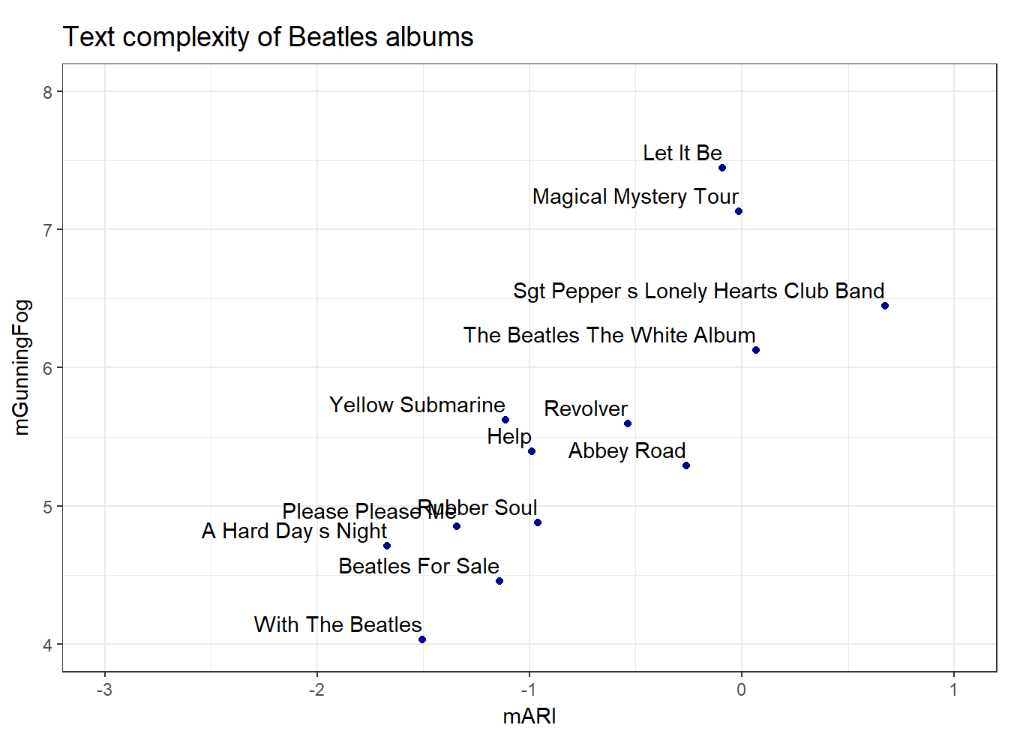
For the complexity metrics I used the ‘syllable’ package, which produces certain text statistics from which these scores can be calculated. The result is in the next chart.
text_complexity <- data.table(album = character(),
                              mGunningFog = numeric(),
                              mARI = numeric())

for(i in 1:nrow(beatles_albums)){
  name <- beatles_albums[[1]][i]
  l <-  list(name)
  temp_lyr <- beatles_lyrics %>%
    filter(album == as.character(name)) %>%
    distinct(text)
  rwstat <- readability_word_stats(temp_lyr[,1])
  l <-  list.append(l, 0.4*(rwstat$n.words/nrow(temp_lyr)) +
                      100*(rwstat$n.complexes/rwstat$n.words))
  l <- list.append(l, 4.71*(rwstat$n.chars/rwstat$n.words) +
                     0.5*(rwstat$n.words/nrow(temp_lyr)) - 21.43)
  text_complexity <- rbind(text_complexity, l)
}

ggplot(data = text_complexity, aes(mARI, mGunningFog)) +
  geom_point(color = "darkblue") +
  geom_text(aes(x = mARI, y = mGunningFog, label = album), hjust=1, vjust=-0.5) +
  theme_bw() + labs(title = "Text complexity of Beatles albums") +
  theme(plot.title = element_text(size = rel(1.25)))  +
  ylim(4,8) + xlim(-3,1)

While the two metrics put the albums in slightly different orders, the trend is obvious. The first albums (Please Please Me, A Hard Day’s Night, With The Beatles) are of fairly simple text, but as time goes by sophistication increases. Let It Be (no. 13) and Abbey Road (no. 12) have fairly high readings by ARI, and Let It Be is the single most complex according to Gunning Fox. Note that Sgt. Pepper (no. 8) is of relatively high complexity: it is the most complex by ARI and the third most complex by Gunning Fog. Remember, Sgt. Pepper is the most dissimilar album compared to the Please Please Me benchmark by cosine similarity.
If we look at the publication dates of these albums (not shown here) we
do see a development in the group’s artistic performance. Four out of
the last five albums (‘Magical Mystery Tour’, ‘The Beatles The White
Album’, ‘Abbey Road’, ‘Let It Be’) are in the top right corner of the
chart, while the first five LPs are in the bottom left.
Summary
This short analysis tries to provide an insight into the carrier of The Beatles through their lyrics. Songs were very simple at the beginning, but as their music got more mature, their lyrics followed on. Measures of text complexity, just as those of similarity, can also reveal the uniqueness of the St. Pepper’s album.
Among the tools, tidytext, syllable, and of course the geniusR packages were used to compile this report.
Codes can be found at https://github.com/peterduronelly/blogcodes/blob/master/02-Text-Complexity-Analysis-Of-Beatles_Lyrics-With-R.R.