One of the things we need to manage in data analysis is recources. When we have large amounts of (‘big’) data this can become a serious issue. One of the cases when we need to consider whether we really need all the data we have is when we have a lot of zeros in our database, and these zeroes happen to be irrelevant for our calculations. Python’s SciPy library has a solution to store and handle sparse data matrices which contain a large number of irrelevant zero values.
In order to demonstrate how this works let’s first import the necessary packages.
import numpy as np
from scipy.sparse import coo_matrix
from scipy.sparse import save_npz
import matplotlib
import matplotlib.pyplot as plt
%matplotlib inline
import random
Where would we come across sparse data? Let’s imagine you are running an e-commerce site where people buy various products. Some poeple buy only one item, others buy multiple products. You want to see how clients are related, or linked, to each other based on their purchase patterns: if some customers buy the same or almost the same set of products, these clients are similar.
Moreover, these linkages create a network clients, and this network can be used for recommendations, coupons, etc. Without going into the details how such a network can be built and used let’s see how we get to sparse data when we analyze buying patterns.
For the sake of simplicity let’s assume that there are 15 clients and 30 products. Each client buys between 2 and 8 pieces of items.
clients = list(range(0,15)) # 15 clients
dic = {} # a dictionary of purchases: keys are clients and values are lists of items bought
for i in range(0,15):
    key = clients[i]
    random.seed(i)
    l = random.sample(range(0,30), random.randint(2,8))
    dic[key] = l
We can print out what itemms clients have purchased.
for key in dic.keys():
    print(dic[key])
[12, 24, 13, 1, 8, 16, 15, 29]
[18, 27, 25]
[27, 1, 2, 29, 11, 5, 23, 21]
[18, 17, 4]
[9, 3, 23]
[8, 23, 11, 25, 22, 28]
[18, 26, 2, 15, 24, 8, 1, 0]
[4, 12, 20, 1]
[11, 12, 4]
[19, 11, 8, 4, 5]
[1, 13, 15, 18, 0, 6]
[27, 17, 29, 24, 14]
[8, 21, 16, 11, 4]
[9, 21, 29, 25]
[19, 22]
Clients No. 0, 2 and 6 have bought eight items, and only one has bought two. Now we can build a matrix of clients where the matrix elements show the number of common items on their shopping history. Each aij element of this matrix tells the number of items bought both by client i and client j . The ith diagonal element shows the number of items bought buy client i. This is going to be a symmetric matrix, of course.
To build the matrix we need to define the row and column indices of the non-zero matrix elements, and the values of the elements. These are going to be lists of equal sizes, which serve as inputs for the sparse matrix. Since the matrix is symmetric, we don’t need to calculate and store the lower diagonal elements to save space.
r = 0 # the index of the row of the matrix
c = 0 # the index of the columns of the matrix
counter = 0
row_indices = [] # row indices of the non-zero values
column_indices = []  # column indices of the non-zero values
matrix_elements = [] # the non-zero values themselves

for key_r in dic.keys(): # key_r is the key for the rows
    x = dic[key_r]
    for key_c in dic.keys(): # key_c is the key for the columns
        if c >= r:
            y = dic[key_c]
            common_set = list(set(x) & set(y))
            common_set_size = len(common_set)
            if common_set_size > 0:
                row_indices.append(r)
                column_indices.append(c)
                matrix_elements.append(common_set_size)
        c = c + 1
    r = r + 1
    c = 0
Once we have the lists we can build the sparse matrix using the coo_matrix function. This function takes numpy arrays as inputs so we need to convert our lists to arrays. When building the matrix we need to add the non-zero elements first, then the indices as a tuple. Finally we need to define the size (shape) of the matrix. The resulting object will be of type scipy.sparse.coo.coo_matrix.
row  = np.array(row_indices)
col  = np.array(column_indices)
val = np.array(matrix_elements)
mx = coo_matrix((val, (row, col)), shape=(15, 15))
We can view the content of the matrix using the .toarray() command.
mx.toarray()
array([[8, 0, 2, 0, 0, 1, 4, 2, 1, 1, 3, 2, 2, 1, 0],
[0, 3, 1, 1, 0, 1, 1, 0, 0, 0, 1, 1, 0, 1, 0],
[0, 0, 8, 0, 1, 2, 2, 1, 1, 2, 1, 2, 2, 2, 0],
[0, 0, 0, 3, 0, 0, 1, 1, 1, 1, 1, 1, 1, 0, 0],
[0, 0, 0, 0, 3, 1, 0, 0, 0, 0, 0, 0, 0, 1, 0],
[0, 0, 0, 0, 0, 6, 1, 0, 1, 2, 0, 0, 2, 1, 1],
[0, 0, 0, 0, 0, 0, 8, 1, 0, 1, 4, 1, 1, 0, 0],
[0, 0, 0, 0, 0, 0, 0, 4, 2, 1, 1, 0, 1, 0, 0],
[0, 0, 0, 0, 0, 0, 0, 0, 3, 2, 0, 0, 2, 0, 0],
[0, 0, 0, 0, 0, 0, 0, 0, 0, 5, 0, 0, 3, 0, 1],
[0, 0, 0, 0, 0, 0, 0, 0, 0, 0, 6, 0, 0, 0, 0],
[0, 0, 0, 0, 0, 0, 0, 0, 0, 0, 0, 5, 0, 1, 0],
[0, 0, 0, 0, 0, 0, 0, 0, 0, 0, 0, 0, 5, 1, 0],
[0, 0, 0, 0, 0, 0, 0, 0, 0, 0, 0, 0, 0, 4, 0],
[0, 0, 0, 0, 0, 0, 0, 0, 0, 0, 0, 0, 0, 0, 2]])
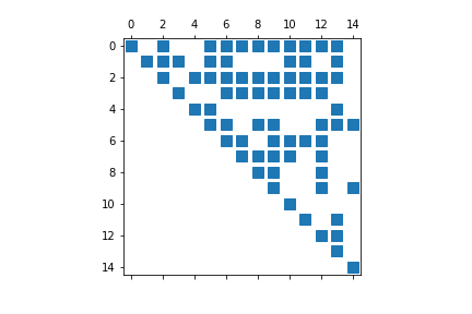
We can also visualize the matrix using the matplotlib library. This visualization shows where the non-zero values are located in the matrix, but it does not make a difference based on their values. All non-zero entries are indicated by the same color.
plt.spy(mx)
plt.show()

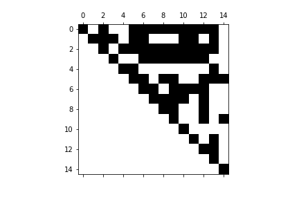
The chart has a slighlty different outlook if we use the matrix as a numpy array, and not as scipy.sparse.coo.coo_matrix object as plot input. The chart is built a little faster and has a different coloring scheme. The visualization, however, does not help much when we have really large amount of data, with thousands of rows and columns in our matrix: the screen resolution will not be able to differentiate between the white and non-white areas. This makes this visulization tool kind of useless in those cases when we really need to use the sparse matrix fuctionality for our resource management.
mx_as_array = mx.toarray()
plt.spy(mx_as_array)
plt.show()

Finally we can save the scipy.sparse.coo.coo_matrix object using the save_npz() command. For later use, the load_npz() command imports the sparse matrix to our project.
save_npz('/path...', mx)
The codes can be find at my github.