Stargazer is a neat tool to present model estimates. It accepts a fairly large number of object-types and creates nice-looking, ready-to-publish outputs of their main parameters. In many cases, however, the default settings do not give us the proper numerical results, and customizing the output is not that straightforward. This is part one in a two-part series on how to customize stargazer.
When I first encountered stargazer I already had a problem with the model outputs the package created: in cross-sectional data the observations are often of different sizes, which leads to heteroskedastic model residuals where simple standard errors are useless for measuring variable significance. Heteroskedasticity requires ‘robust’ standard errors to calculate p-values, but there is no flag in stargazer to switch from simple to robust standard errors. The same problem emerges with panel models, where, for basically the same reason, ‘clustered’ standard errors need to be calculated and applied. If the output is based on the wrong errors, then the model cannot be presented with stargazer. However, I haven’t been able to find any other package which can create such a tidily formatted model output.
The good news is that stargazer can be fed externally with the right standard errors, which then results in the proper output. This post shows you how.
library(wbstats) # to retrieve World Bank development data to demonstrate stargazer functionalities
library(dplyr)
library(data.table)
library(plm)
library(stargazer) # this is the package what we are interested in
library(sandwich) # to calculate robust and clustered stanard errors
library(pander)
I am using the wbstats package to download data from the World Bank development database. As countries are of different sizes, running a regression of any kind requires ‘non-standard’ standard errors to calculate variable significance. We will do a cross-section and a panel regression to demonstrate stargazer options.
In a simple model I try to explain the number of patent applications in a country with real PPP GDP and population size. The goal of this exercise is not about building the right model, the regressions are for demonstrational purposes only.
data <- wb(indicator = c("NY.GDP.MKTP.PP.KD", # WB (World Bank) code for PPP GDP per capita in 2011 $
                         "IP.PAT.RESD", # WB code for patent applications by residents
                         "SP.POP.TOTL"), # WB code for population
                       startdate = 2000,
                       enddate = 2015)

countries <- wbcountries()

data <- merge(data, countries[c("iso2c", "region")],
                          by = "iso2c", all.x = TRUE)
data <- subset(subset(data, region != "Aggregates"))

data$indicatorID[data$indicatorID == "NY.GDP.MKTP.PP.KD"] <- "GDP"
data$indicatorID[data$indicatorID == "IP.PAT.RESD"] <- "patent_applications"
data$indicatorID[data$indicatorID == "SP.POP.TOTL"] <- "population"

data <- dcast(data, iso2c + country + date + region ~ indicatorID,  value.var = 'value')

names(data)[names(data) == "date"] <- "year"
data$year <- as.numeric(data$year)
data <- data %>%
  select(-iso2c, -region)

data$population <- data$population / 10^6 # some rescaling
data$GDP <- data$GDP / 10^9

data <- data[complete.cases(data),]
Without going into the details of the wbstat package we end up with a data frame where country and year are in columns 1 and 2, and the three other variables (GDP in USD bn, patent applications and population in millions) are in columns 3-5. (This is the default format for panels in R.) The panel is only slightly unbalanced: even if a large number of observations is missing the observations with missing values will not make much trouble. (The punbalanced() command measures how unbalanced the panel is, but this is also beyond the scope of this analysis.)
Robust Standard Errors
Now let’s do a simple cross sectional regression for 2011.
linear_regression <- lm(formula = patent_applications ~
                          GDP + population,
                        data = data %>% filter(year == 2011))
Now comes the trick! The vcov() function in the sandwich package calculates the robust standard errors that we need for coefficient testing when model residuals are heteroskedastic. Vcov gives us the variable covariance matrix, which measures co-dependencies between the variables. It’s diagonal elements are the variances of the variables, which are used for variable importance testing. We need to extract these diagonal elements, take their square root, and feed them into stargazer.
robust_standard_errors <- vcov(linear_regression, sandwich)
robust_standard_errors <- sqrt(diag(robust_standard_errors))
Our standard erorrs are the following.
df = data.frame(robust_standard_errors)
pander(df)

This is the input We can feed into stargazer using the ‘se’ option from the method’s parameter set. It is important to note that the object containing the errors should be given as a ‘list’, even if we only show one model with stargazer.
stargazer(linear_regression, title = "Linear regression",
          se = list(robust_standard_errors),
          type = "html", out = "linear regression.html")
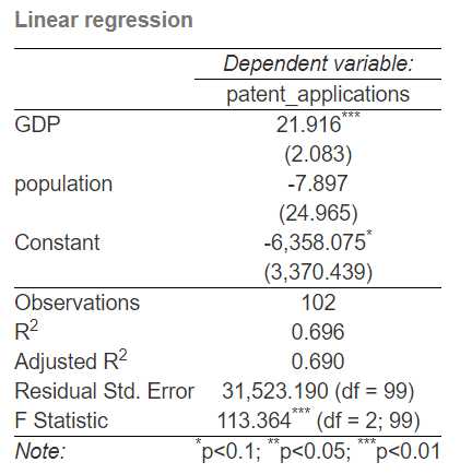
The ‘out’ parameter in stargazer defines the name of the output file we create, and ‘type’ defines the file’s extension. Once we run the command we will get the following (kind of) neatly formatted output which includes our externally fed standard errors and the relevant t-statistics based on those standard errors.

Clustered Standard Errors
Now let’s do two panel regressions using the whole dataset: a fixed-effects (FE) model and a first difference (FD) model. We will include both models in our stargazer output for which we need to supply two sets of standard errors. What is robust standard errors in cross sectional regressions is ‘clustered’ standard errors in panels. This time the vcovHC() function will take care of the standard errors.
First the two panels. As I said before, model validity is not an issue here, I just want to have standard errors.
p_data = pdata.frame(data) # we need to create a 'panel data frame' for panel regressions

fe_regression <- plm(patent_applications ~ GDP + population, # FE model
                     data = p_data,
                     model = "within",
                     effect = "twoways")

fd_regression <- plm(diff(patent_applications) ~ diff(GDP, lag = 2) + # FD model
                       diff(diff(GDP), lag = c(0:1)) +
                       diff(population, lag = 2) + diff(diff(population), lag = c(0:1)),
                     data = p_data,
                     model = 'pooling')
From these two models we extract the clustered standard errors the same way, but now with the vcocHC() function which handles clustered errors in panel models.
clustered_standard_errors_fe <- vcovHC(fe_regression, type = "HC0", cluster = "group")
clustered_standard_errors_fe <- sqrt(diag(clustered_standard_errors_fe))

clustered_standard_errors_fd <- vcovHC(fd_regression, type = "HC0", cluster = "group")
clustered_standard_errors_fd <- sqrt(diag(clustered_standard_errors_fd))
Once we have the standard errors ready, we add them as stargazer parameters. Note, that they are given as lists again.
stargazer(fe_regression, fd_regression, title = "Panel regressions",
          se = list(clustered_standard_errors_fe, clustered_standard_errors_fd),
          type = "html", out = "panel regression.html")
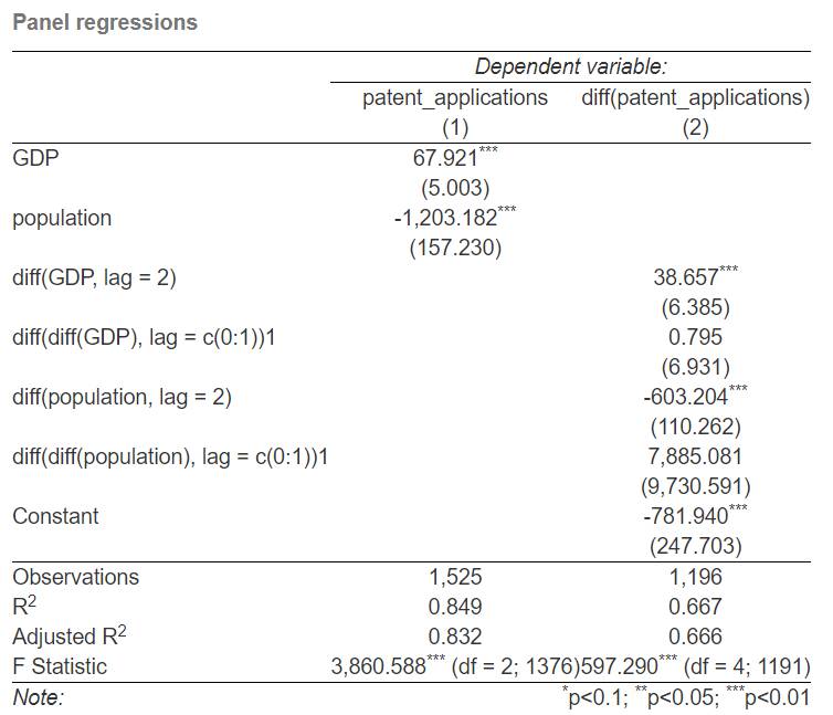
Now the stargazer output looks like this.

We have everything we need in our model output, and stargazer uses the proper standard error set for both models to coefficient testing. We even have more than we really need, and the labels are kind of messy. There are more options to customize stargazer and make it look better, but it is the subject of the other post on stargazer.
Codes at the usual place.