Clustering is one of the well-known unsupervised learning tools. In the standard case you have an observation matrix where observations are in rows and variables which describe them are in columns. But data can also be structured in a different way, just like the distance matrix on a map. In this case observations are by both rows and columns and each element in the observation matrix is a measure of distance, or dissimilarity, between any two observations. This structure can also serve as a basis for clustering, just as you can cluster cities based on the respective distances between any two of them.
When I first encountered this problem I did not find a solution in the standard scikit-learn library which you automatically call when doing a clustering exercise. SciPy, fortunately, has a solution. Let’s see how it works!
import pandas as pd
import numpy as np
import matplotlib.pyplot as plt
import math
from scipy.cluster.hierarchy import linkage, dendrogram, fcluster
The exercise is done on the hundred largest US cities. The list is coming from https://gist.github.com/Miserlou/c5cd8364bf9b2420bb29#file-cities-json in a very neat format. (Thanks to Rick Jones for the data!) It includes not only the city, the state and the population but the latitude/longitude coordinates of the cities wich can be used to calculate an approximate distance measure between the cities.
filepath = ...
cities = pd.read_json(filepath)
cities.head()

By selecting the top 100 cities we get sufficient number of observations and we are still able to interpret the result through simple visualization.
top100 = cities[0:100]

fig = plt.figure()
ax = fig.add_axes([0,0,1,1])
ax = plt.scatter(top100["longitude"], top100["latitude"])
plt.title("The Locations of the 100 Largest US Cities")
plt.show()

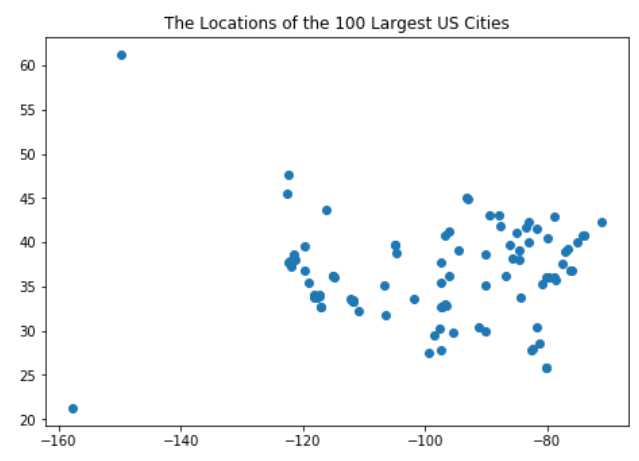
A more fancy map could be generated using the folium package but this simple scatter plot is sufficient for our purposes. As all real, non-simulated data, our city dataset does not show a very obvious pattern. Cities are scattered seemingly randomly on the map, and we have two outliers, Anchorage on the North-West and Honolulu on the South-West, which are very far from all other points.
Now let’s calculate the distances between the cities using the geopy package. The distances can be interpreted as dissimilarities: the larger the distance between two observations the less similar they are. This is may literally not be the case with cities (two distant cities can easily be alike), but when we think in a more abstract space the concept makes sense. Also, city clusters are interpreted in terms of geographical distances, so using them in this exercise helps us understand the method and its results.
distance_matrix = np.empty(shape = [100,100])

for i in range(100):
    for j in range(100):
        coords_i = (top100.iloc[i]["latitude"], top100.iloc[i]["longitude"])
        coords_j = (top100.iloc[j]["latitude"], top100.iloc[j]["longitude"])
        distance_matrix[i,j] = geopy.distance.vincenty(coords_i, coords_j).km
Before we move on to build the clusters and visualize the results let’s create a list of city names where the name of each city is followed by the state. This helps us interpret the cluster tree, the so-called ‘dendrogram’.
cities["city, state"] = top100["city"].map(str) + ", " + top100["state"]
citynames = cities["city, state"][0:100].tolist()
citynames[0:10]
[‘New York, New York’,
‘Los Angeles, California’,
‘Chicago, Illinois’,
‘Houston, Texas’,
‘Philadelphia, Pennsylvania’,
‘Phoenix, Arizona’,
‘San Antonio, Texas’,
‘San Diego, California’,
‘Dallas, Texas’,
‘San Jose, California’]
No we get to the most important part! The meat of the module is the linkage function (scipy.cluster.hierarchy.linkage(…)), which runs the actual clustering algorithms. It can handle both an n x n distance matrix and a regular n x m observation matrix as input. If we form the clusters on a distance matrix, we need its condensed format: the upper diagonal elements (excluding the diagonals) have to be converted into a vector (a list) with a length of n(n-1)/2. The output is a (n-1)x4 NumPy array Z, called linkage matrix, which contains the hierarchical clustering algorithm’s encoded results.
Each row in Z represents one iteration. In each row i, clusters with indices of Z[i,0] and Z[i,1] are combined in a new cluster, based on the distance between them which is in Z[i,2]. The number of elements in the newly formed cluster is Z[i,3].
This is a hierarchical clustering method: we start with elementary clusters (the observations) which are merged into larger and larger clusters. At the end all observations form a single cluster.
Clusters contain observations which are close to each other. Closeness can be defined between observations (cluster elements) and the clusters themselves. To calculate distances between two clusters we need to define two parameters:
We need to define a distance metric, which measures the distances between the elements of one cluster and the elements of the other cluster. The default is the Euclidean distance which is sufficient for our clustering project.
We also need to define a method to sum up the distances between the individual elements of two clusters to come up with a single value for the distance between them. Just as in the case of the measures of central tendency, we are looking for the typical distance between the elements of any two clusters. The method sets how this typical distance is defined.
While the distance metric can also make a difference, the most important parameter in cluster formation is the method. There are various options (methods) to define how far two clusters are from each other: the distance between the two closest elements, or the one between two most distant ones, or some sort of average of the distances between elements of cluster a and cluster b, etc. If cluster a and cluster b have u and v number of elements, respectively, we will have u*v distances which we can use to find the distance between clusters a and b. This is the modeler’s choice and, as I will show it later, it can create markedly different cluster structures. The methods are very well explained in the SciPy documentation and I urge you to check it out. At this point, however, we only need to keep in mind that the method is the most important parameter we need to set.
The most evident difference between clustering methods is how they handle outliers (Anchorage and Honolulu). We will see that merging the mainland and the coastal areas will be completely different in some cases.
And now comes the trick! SciPy does not use the whole dissimilarity matrix for the calculations, only a list of the upper diagonal elements. The length of the list is n(n-1)/2 and SciPy automatically calculates the number of observations it needs to cluster.
l = [] # upper triangular elements of the distance matrix

for i in range(0, distance_matrix.shape[0]):
    for j in range(i + 1, distance_matrix.shape[0]):
        l.append(distance_matrix[i,j])

Z = linkage(l, method="ward") # this is the meat of the thing!
Once we have the linkage matrix, which is basically a log of which observation or cluster got merged in each step, we can visualize the results.
fig = plt.figure(figsize=(25, 10))
plt.title("Hierarchical Clustering Dendrogram\nLinkage = ward")
plt.xlabel('city, state')
plt.ylabel('distance')
dn = dendrogram(Z,
               labels = citynames,
    leaf_rotation=90.,
    leaf_font_size=10.,
    show_contracted=True)
plt.show()

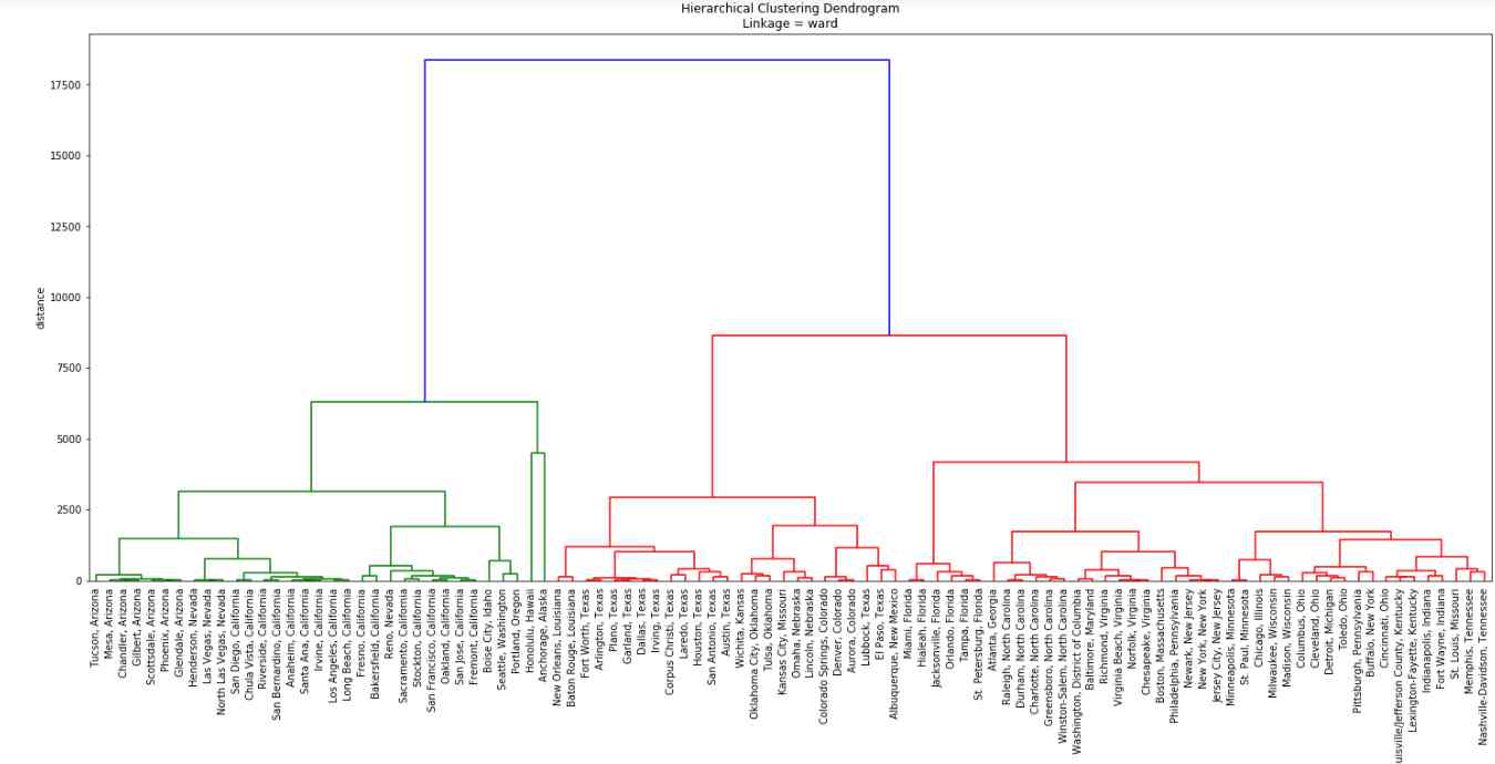
First we used the ‘ward’ method which is an optimization algorithm: it aims to minimize within-cluster variance. Cities belong to two major clusters: the ones with green linkages can be called ‘The West’, while the ones with red linkages can be considered ‘The East’ or ‘East + Midwest’. Our outliers (Anchorage and Honolulu) belong to the West, which makes sense, and they form a cluster together before being linked to the other Western cities. Before they are linked, however, mainland Western/West Coast cities are merged into clusters at higher and higher levels of aggregation. Only then come the two overseas cities.
Cities in Arizona are merged into their own clusters, then Nevada and California. Boise City, Idaho goes to Nevada/California after being merged with the cluster formed by Seattle and Portland. Everything else belong to the East Coast, including cities in Minnesota, Wisconsin and Texas. The dendrogram is sort of ‘smooth’ or ‘balanced’, thanks to the algorithm’s variance minimalization.
The vertical axis shows the distance, or the level of dissimilarities between the clusters. The longer the vertical lines the more dissimilar the two clusters which are merged in that step. The lenght of the two vertical blue lines shows that this method considers the West Coast, which includes the outlier cities, to be very different from everything else.
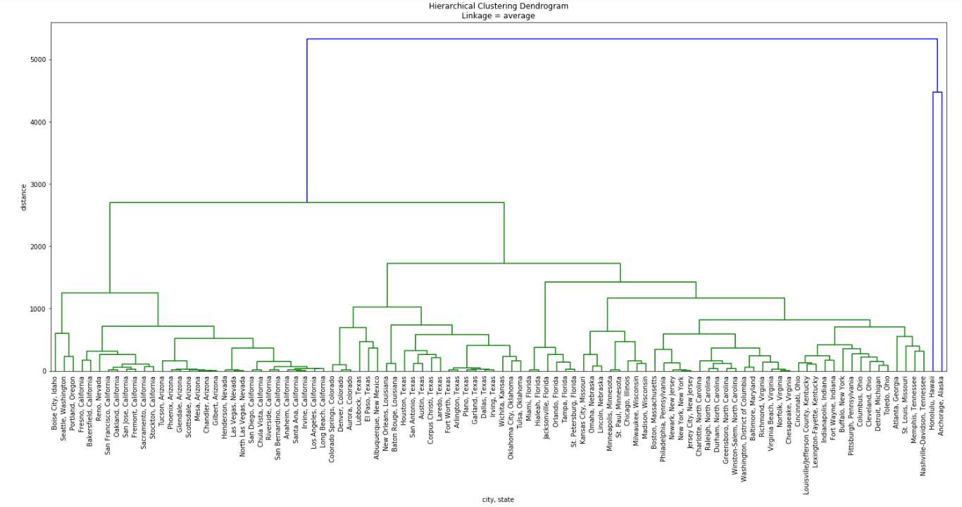
The structure changes a lot when cluster distances are defined as the average distance between the members of the two clusters. The fact that cluster formation is not variance-optimized results in an unbalanced-looking tree.
Z = linkage(l, method="average")

fig = plt.figure(figsize=(25, 10))
plt.title("Hierarchical Clustering Dendrogram\nLinkage = average")
plt.xlabel('city, state')
plt.ylabel('distance')
dn = dendrogram(Z,
               labels = citynames,
    leaf_rotation=90.,
    leaf_font_size=10.,
    show_contracted=True)
plt.show()

The most visible difference, as I mentioned before, is how the outliers are handled. Here they are merged with other mainland cities only at the end, only after the other 98 cities have been joined together. There is more emphasis on their uniqueness than before, when within-cluster variance ruled cluster formation. East Coast and West Coast are made up from mostly the same cities as before, but their aggregation, from individual cities to larger and larger formations has a somewhat different profile.
It is also interesting to see how the trio of Boise City and Seattle & Portland is linked to Arizona and California. In the ‘ward’ optimization mechanism they are merged with California before they together are put together with Arizona. In this latter case Arizona, California and Nevada are merged before the trio of Boise, Seattle & Portland joins them as the last West Coast areas.
No one is better than the other, and both the nature of the data and the target of the modeling exercise are important in selecting the best method. In the case of the US cities, for example, if we think that the mainland cities share more with each other than with Anchorage or Honolulu, ‘average’ is a better choice. If we simply want a split into East and West, then ‘ward’ will be our method.
As a summary: clustering is possible in Python when the data does not come as an n x p matrix of n observations and p variables, but as an n x n dissimilarity or distance matrix. The home of the algorithm is the SciPy package, and depending on the method, we can have very different results.
The codes are at the usual place.