Bootstrap sampling is a widely used method in machine learning and in statistics. The main idea is that we try to decrease overfitting and the chance of myopic tree-building if run our algorithm multiple times using the same data, but always taking a different sample with repetitions from our original data. (For instance, random forest builds the trees using repeated bootstrap samples.) On a machine learning class one of my class mates asked what percentage of the original data shows up in the bootstrapped sample. Let’s have a look!
import random
import matplotlib.pyplot as plt
%matplotlib inline
import pandas as pd
In bootstrap samples we select elements from our original sample in the same number as the size of the original data at hand using repetitions. This is a poster case for Central Limit Theorem, thus the expected value of our sample mean will be bang in line with the mean of the original data.
Let’s have a dataset of 1,000 observations, from which we take 10,000 samples of 1,000 elements. This number of sampling helps us visualize and calculate our sample properties.
When bootstrapping, some original observations show up multiple times and some others will be missing from the bootstrapped samples. We are about finding the number of distinct elements in the bootstrapped samples. If the samples are lists, then turning these lists into sets helps us calculate the number of distinct elements, since sets don’t have the same value more than once.
sample_sizes = []
for i in range(10000):
    sample = []
    for j in range(1000):
        sample.append(round(random.randint(1,1000)))
    sample_sizes.append(len(set(sample)))
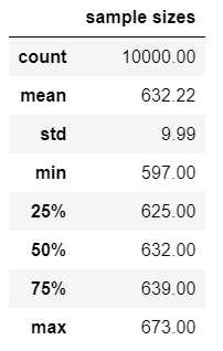
Turning the sample size list into a data frame we can easily get the most basic statistics.
df = pd.DataFrame(sample_sizes)
df.columns = ["sample sizes"]
df.describe().style.format('{:.2f}')

We have taken 10,000 samples of 1,000 observations with repetitions from the 1,000 observations. On average, 632 observations show up in the bootstrapped samples, and this number is between 625 and 639 in the half of the samples. These results are extremely stable: if you run this simulation multiple times the average will always be 632.
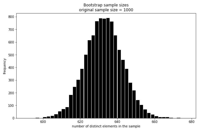
It shouldn’t come as a surprise that the distribution of the number of distinct elements is almost perfectly normal.
fig = plt.figure(figsize = (10,6))

plt.hist(df["sample sizes"], bins = list(range(590, 680, 2)), rwidth=0.9, color = 'k')
plt.title("Bootstrap sample sizes\noriginal sample size = 1000")
plt.xlabel("number of distinct elements in the sample")
plt.ylabel("frequency")
plt.show()

Codes are at the usual place.